VC Theory and PAC Learning

Learning from Samples

The goal of learning from samples is to learn an unknown function $f$ from as few samples as possible. We receive inputs $x$ drawn i.i.d. from a distribution and query the oracle (a black box). The oracle outputs the value $f(x)$. From these input-output pairs, we want to reconstruct or approximately learn the function.

Let us take a specific example and learn a toy function under specific conditions.

Suppose $\mathcal{X}$ is a finite domain, the inputs are drawn uniformly from $\mathcal{X}$, and $f : \mathcal{X} \to \{-1,+1\}$. We are promised that $f$ is either constant on the entire domain or assigns each label to exactly half of the domain. That is, either

$$\begin{aligned} \text{A.}\quad &\exists c \in \{-1,+1\} \quad \text{such that} \quad f(x)=c \quad \forall x \in \mathcal{X}, \\[4pt] &\text{or} \\[4pt] \text{B.}\quad &\left|f^{-1}(-1)\right| = \left|f^{-1}(+1)\right| = \frac{|\mathcal{X}|}{2}. \end{aligned}$$

Now, we have two options, and I need to figure out which kind of function the oracle represents. I draw samples and look at their outputs. The outputs may be different, or they may all be the same. If I observe both $+1$ and $-1$, I can immediately say that the function is balanced because of the promise. If all the outputs are the same, however, I cannot be certain. My learning rule will declare the function constant in that case, so all I can talk about is the probability that this decision is wrong.

For example, let us say that I have drawn three samples and all are in the $+1$ class. Can I say that the function is constant? No. A balanced function could also produce those three outputs. Nor can I say for sure that it is balanced and that drawing more samples will reveal this. My whole issue is to figure out how many samples I need before making a decision, so I must choose that number in advance.

Then comes the idea of probability. If the function is balanced, each draw has probability $1/2$ of producing either label. Therefore, the probability that three draws are all $+1$ is

$$\left(\frac{1}{2}\right)^3 = \frac{1}{8}.$$

The same is true for three outputs that are all $-1$. Thus, the probability that all three outputs are the same, causing my learning rule to mistake a balanced function for a constant one, is

$$2\left(\frac{1}{2}\right)^3 = \frac{2}{8} = \frac{1}{4}.$$

So, now comes the big question: how much risk of being fooled by the sampled observations can I afford? I shall call this limit $\delta$, where $0 < \delta < 1$.

If I draw $n$ samples, the probability that a balanced function produces only one label is

$$2\left(\frac{1}{2}\right)^n = 2^{1-n}.$$

Therefore, I will choose enough samples that

$$2^{1-n} \leq \delta.$$

This makes sure that the probability of my learning rule being fooled by the sampled observations is at most $\delta$.

Equivalently, I need

$$n \geq 1 + \log_2\left(\frac{1}{\delta}\right).$$

Since the number of samples must be an integer, the smallest such choice is $n = \left\lceil 1 + \log_2(1/\delta) \right\rceil$.

We can distinguish between case A and case B with probability atleast $1-\delta$ using $O(log\frac{1}{8})$ queries. $\delta$ $\ge 0$ under finite no. of samples.

Goals in Learning Theory

Given a function $f : \mathbb{X} \to \mathbb{R}$, and knowing that $f \in \mathcal{F}$, where $\mathcal{F}$ is a set of structured functions, we want to learn $f$ using as few queries as possible to the black box, with a success probability of at least $(1-\delta)$.

Ideally, we want to learn $f$ exactly, but that is quite hard to achieve.

Here, learning means that, with probability at least $1-\delta$ over the sampled observations, your algorithm will output some $\tilde{f} \in \mathcal{F}$ such that

$$\mathbb{P}_{x}(\tilde{f}(x) \neq f(x)) \leq \epsilon.$$

This is called $(\epsilon, \delta)$-PAC learning. We need to figure out $\tilde{f}$. For this, we need to know the sample complexity. Sample complexity is denoted by

$$\mathcal{s}(\epsilon, \delta)$$

which is the number of i.i.d. samples from $\mathbb{X}$ I need to learn $f$ with these guarantees. If the sample complexity is higher, then the function class is harder to learn.

Inner product, Affine functions and Hyperplanes

Inner Product

Let us say $\mathbb{X}\subseteq \mathbb{R}^{N}$. Given two points $\bar x, \bar y \in \mathbb{R}^{N}$. $\langle \bar x, \bar y \rangle$ denotes the inner product between $\bar {x} \quad \& \quad \bar {y}$. Inner product is defined as

$$\langle \bar x, \bar y \rangle = \sum_{i=1}^{N}(\bar x_{i} \bar y_{i})$$

where $\bar x = (\bar x_1, \bar x_2, \dots, \bar x_N)$ and $\bar y = (\bar y_1, \bar y_2, \dots, \bar y_N)$

Affine functions over $\mathbb{R}^{N}$

An affine function $\mathcal{f_{\bar a, b}}(\bar x)$ is defined as

$$\mathcal{f_{\bar a, b}}(\bar x) = \langle \bar a, \bar x \rangle + b$$

where $\bar a \in \mathbb{R^{N}} \quad \& \quad b \in \mathbb{R}$

Hyperplanes

An affine function assigns a real value to every point in $\mathbb{R}^N$. A natural question to ask is: what is the set of points that receive the same value under this function? In particular, the set of points where the affine function evaluates to zero forms a geometric object known as a hyperplane.

Given an affine function

$$\mathcal{f}_{\bar a,b}(\bar x)=\langle \bar a,\bar x\rangle+b,$$

the hyperplane induced by this affine function is the set of all points whose function value is zero. Formally,

$$H=\left\{\bar x\in\mathbb{R}^N:\langle \bar a,\bar x\rangle+b=0\right\}.$$

The hyperplane partitions the space into two half-spaces:

$$\langle \bar a,\bar x\rangle+b>0$$

and

$$\langle \bar a,\bar x\rangle+b<0.$$

Thus, every point in $\mathbb{R}^N$ either lies on the hyperplane or belongs to one of the two half-spaces.

Radon's Theorem

The theorem is referred from convex geometry.

Let $P_{1},P_{2},P_{3} \dots P_{N},P_{N+1},P_{N+2}$ be points in $\mathbb{R}^{N}$. Then $\exists$ two partitions $S_{1}$ and $S_{2}$ of the aove points such that $S_{1}$ and $S_{2}$ of the above points cannot be separated by a linear classifier. This means that we can make such partitions for which we can never make a linear classifier to partition them. (think of yin-yang diagram).

$$S_{1} \cap S_{2} = \phi \\ S_{1} \neq \phi \\ S_{2} \neq \phi \\ S_{1} \cup S_{2} = {P_{1},P_{2},P_{3} \dots P_{N},P_{N+1},P_{N+2}}$$

Proof

Using the fact that any $N+1$ vectors in $\mathbb{R}^{N}$ are linearly DEPENDENT, we can show that $\quad \exists \quad \lambda_{1}, \lambda_{2}, \dots, \lambda_{N+2}$ in $\mathbb{R}$ not all $\lambda$ being zeros, such that

$$\sum_{i=1}^{N+2}(\lambda_{i} P_i) = 0\\ \text{and}\\ \sum_{i=1}^{N+2} (\lambda_i) = 0$$

Let us say $P_1$ is origin and $v_i = P_{i+1} - P_1 , \forall i \in [N+1]$ Since

$$\sum_{i=1}^{N+2}\lambda_i=0,$$

there must exist both positive and negative coefficients (otherwise all the coefficients would have to be zero).

Define

$$L^-=\{\,i\mid \lambda_i<0\,\}, \qquad L^+=\{\,i\mid \lambda_i>0\,\}.$$

Now partition the given points into

$$S_1=\{P_i\mid i\in L^-\}, \qquad S_2=\{P_j\mid j\in L^+\}.$$

Using

$$\sum_{i=1}^{N+2}\lambda_iP_i=0,$$

we obtain

$$\sum_{i\in L^+}\lambda_iP_i = \sum_{j\in L^-}(-\lambda_j)P_j.$$

Let

$$\alpha = \sum_{i\in L^+}\lambda_i = \sum_{j\in L^-}(-\lambda_j),$$

where the equality follows from

$$\sum_{i=1}^{N+2}\lambda_i=0.$$

Dividing both sides by $\alpha$, we get

$$\sum_{i\in L^+}\frac{\lambda_i}{\alpha}P_i = \sum_{j\in L^-}\frac{-\lambda_j}{\alpha}P_j.$$

Notice that all the coefficients on both sides are non-negative and sum to $1$. Hence, both sides represent convex combinations of points in $S_1$ and $S_2$, respectively.

Therefore, there exists a point that belongs to both convex hulls. Hence,

$$\operatorname{conv}(S_1)\cap\operatorname{conv}(S_2)\neq\varnothing.$$

Since two sets whose convex hulls intersect cannot be separated by a linear hyperplane, the partitions $S_1$ and $S_2$ cannot be separated by a linear classifier.

VC Theory

VC Theory is one of the foundational theories in learning.

(As of now, I am very new to this and cannot appreciate VC Theory correctly, but soon I shall rephrase the VC Theory).

Let us introduce the Universe and Ranges.

We denote Universe with '$\mathbb{X}$' and Ranges with '$\mathcal{R}$'.

$$(\mathbb{X},\mathcal{R})$$

where, $\mathcal{R} \subseteq 2^{\mathbb{X}}$. $\mathcal{R}$ is the collection of subsets of the universe. This tuple together is called a set system.

Projection

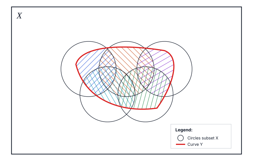
Geometrically, the projection is obtained by restricting every range in $\mathcal{R}$ to the subset $\mathbb{Y}$. Thus, each projected range is the intersection $\mathcal{S}\cap\mathbb{Y}$, and the collection of all such intersections forms $\mathcal{R}_{\mathbb{Y}}$.

Example

Let us understand all this using a small emperical example. Let us say my universe is $\mathbb{X} = \{1,2,3,4\}$ and my ranges are $\mathcal{R} = \{\{1,2\}, \{2,3\},\{1,2,3\}, \{1,3,4\}\}$, where

$$\begin{align} \mathcal{S_1} &= \{1,2\} \\ \mathcal{S_2} &= \{2,3\} \\ \mathcal{S_3} &= \{1,2,3\} \\ \mathcal{S_4} &= \{1,3,4\} \end{align}$$

Each $\mathcal{S_i}$ is a subset of $\mathbb{X}$

If I collect all those \mathcal and store in a set, i.e.,

$$\mathcal{R} = \{\mathcal{S_1}, \mathcal{S_2}, \mathcal{S_3}, \mathcal{S_4}\}$$

it is called family of ranges or simply ranges ($\mathcal{R}$). The tuple $(\mathbb{X}, \mathcal{R})$ is called a set system.

Now, choose a subset $\mathbb{Y} = \{1,2,3\} \subseteq \mathbb{X}$. Now interseting this $\mathbb{Y}$ with each $\mathcal{S_i}$, we get the following:

$$\begin{align} \mathcal{S_1} \cap \mathbb{Y} &= \{1,2\} \\ \mathcal{S_2} \cap \mathbb{Y} &= \{2,3\} \\ \mathcal{S_3} \cap \mathbb{Y} &= \{1,2,3\} \\ \mathcal{S_4} \cap \mathbb{Y} &= \{1,3\} \end{align}$$

If we collect them and store in a set $\mathcal{R_\mathbb{Y}}$, we get

$$\mathcal{R_\mathbb{Y}} = \{\{1,2\}, \{2,3\}, \{1,2,3\}, \{1,3\}\}$$

and this is the $\mathbf{PROJECTION}$.

Shattering

Now let us ignore $\mathbb{X}$ and look only at $\mathbb{Y}$ and see what all are the subsets of $\mathbb{Y}$?

$$2^{\mathbb{Y}} = \{\emptyset, \{1\}, \{2\}, \{3\}, \{1,2\}, \{1,3\}, \{2,3\}, \{1,2,3\}\}$$

Let us now compare $2^{\mathbb{Y}}$ with $\mathcal{R_\mathbb{Y}}$ and see, how do they differ.

$$\begin{align} \mathcal{R_\mathbb{Y}} &= \{\{1,2\}, \{2,3\}, \{1,2,3\}, \{1,3\}\}\\ 2^{\mathbb{Y}} &= \{\emptyset, \{1\}, \{2\}, \{3\}, \{1,2\}, \{1,3\}, \{2,3\}, \{1,2,3\}\} \end{align}$$

We can see that $\mathcal{R_\mathbb{Y}} \subset 2^{\mathbb{Y}}$ and $\mathcal{R_\mathbb{Y}} \neq 2^{\mathbb{Y}}$. This means that the projection of $\mathcal{R}$ onto $\mathbb{Y}$ does not cover all possible subsets of $\mathbb{Y}$. In other words, the set system $(\mathbb{X}, \mathcal{R})$ does not shatter the subset $\mathbb{Y}$

VC Dimension

We denote the VC dimension of a set system $(\mathbb{X}, \mathcal{R})$ as $\text{VC}(\mathbb{X}, \mathcal{R})$ or simply $\text{VC}(\mathcal{R})$.